Benchmarking Libraries and Averaging Trackers

This article explores a powerful tracker/resource combination that’s commonly used to estimate impacts such as energy or emissions when activity data regarding actual resource consumption is not available. In these cases, Scope 5 can estimate resource consumption by tracking proxies such as facility area or number of employees. These data can then be converted to resource consumption (and ultimately energy, emissions and other impacts) using benchmark figures that are part of conversion factors in Scope 5’s benchmark resource libraries.

We’ll discuss this concept in depth in the following paragraphs. While you may find this level of detail helpful, there is one concept that is important to be aware of:

Until recently (v. 7.0.8), when relying on benchmark resource libraries, it was important that the reporting period conformed to the assumed benchmark period in any benchmarking resource library used (typically one year). It is now possible to run reports for arbitrary time spans so long as the resources used are configured with their assumed benchmark period. This is now the case for benchmark resource libraries that are maintained by Scope 5. If you wish to configure your own benchmark resources and support arbitrary reporting periods, please contact your Scope 5 account manager to help configure the resources appropriately.

To understand in further detail how Scope 5 applies benchmark resources, read on.

In the most common scenario, Scope 5 tracks activity data such as electricity or fuel consumed by summing that activity data over time. The tracker/resource combination of interest in this article averages data over time. As such, the math used to convert activity data to impact data differs slightly. 

Summing Resource/Tracker Combination

First - let’s take a quick look at the math for standard summing trackers. For these, each activity record quantifies an amount of some activity that has occurred since the previous activity record  (for accruing trackers) or that occurs until the subsequent activity record (for ongoing trackers). Simply summing activity across a group of activity records quantifies the total activity occurring over the time period spanned by the group of records. This is illustrated in Figure 1:

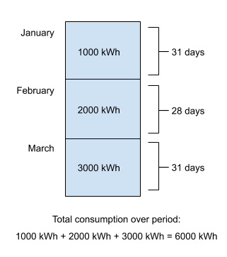
Figure 1 - Summing Activity Records

 

Averaging Resource/Tracker Combination

For averaging trackers, the math is different. For these, activity records usually represent an average metric of some sort, that starts at some time and persists until the next activity record. Such averaging trackers are usually configured as ongoing trackers but are occasionally configured as accruing trackers (in which case activity records represent average values that have been in place since the previous record). Examples of typical averaging metrics include facility area or number of employees. It doesn’t make sense to sum averaging records to roll them up over time. Rather, these records tend to be averaged over time, weighted by the duration over which each record’s average value persists. The three records illustrated in Figure 2 each quantify a facility’s area at the start of a period. The rolled up weighted average quantifies the average area over the three periods. Area values contribute to the rolled up average in proportion to their duration.

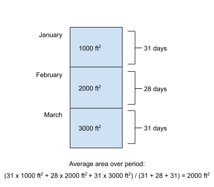
Figure 2 - Averaging Activity Records

Both Tracker Types are Useful

Both tracker types are useful. By rolling up activity records of the summing tracker type, we’re able to make statements like:

Over the three months spanning January, February and March, we used a total of 6000 kWh of electricity.

When rolling up activity records of the averaging tracker type, we can make statements like:

Over the three months spanning January, February and March, the average facility area was 2000 ft².

Benchmarking Resources

Besides providing useful rollups in themselves, averaging trackers can be used to drive resources in benchmarking libraries. Consider for example, the CBECS libraries. These libraries quantify an average expected consumption based on an average intensity metric. For example, a CBECS resource might tell us how much electricity can be expected to be consumed when operating an office of a certain area, over a certain period of time. Thus, if we know the average office area over a certain period, we can estimate the amount of electricity consumed over that period. 

But, whereas the math used to rollup results from summing trackers is fairly straightforward, the math used to roll up results from these kinds of averaging trackers is a little more subtle and complicated. We’ll take a look at it here.

First, it’s important to note the distinction between activity on the one hand and impact metrics on the other. The two examples illustrated previously quantified activity - kWh used and square feet of facility area. In the following discussion, we’ll look at quantifying impact metrics. Impact metrics are derived from activity using conversion factors. Conversion factors are defined by resources and are applied to the activity records belonging to the corresponding trackers. 

Calculating Impact Metrics for Summing Trackers

A common resource might be used by electricity trackers and would contain a conversion factor to convert from kWh of electricity (the activity) to lbs. of CO₂e emissions (the impact metric). Applying this concept to the electricity consumption illustrated in Figure 1, and assuming a conversion factor of 1.2 lbs CO₂e per kWh, we can calculate the total CO₂e emissions for the period January through March:

6000 kWh * 1.2 lbs CO₂e/kWh = 7200 lbs. CO₂e

Calculating Impact Metrics for Averaging Trackers

As mentioned previously, the averaging tracker illustrated in Figure 2 can be combined with a resource from a benchmarking library to estimate consumption (and corresponding impacts). A sample resource from a CBECS library might include a conversion factor that tells us that a typical office in a certain climate zone can be expected to use 11 kWh of electricity per square foot of office area. Applying this conversion factor to the average area calculated in Figure 2, we get:

2000 ft² * 11 kWh/ft² = 22,000 kWh

But there’s an important nuance missing from this calculation - the benchmarking conversion factor quantifies electricity consumption per ft² over a specific time period. In the case of the CBECS libraries, resources quantify average electricity consumption per ft² over a period of one year. So - although the calculation above yielded 22,000 kWh of electricity consumed, that result assumes that the office was operated for an entire year and that the average office area over that year was 2000 ft². To quantify the electricity consumed over the 90 day period illustrated, we need to prorate the result as follows:

elec₉₀ =  elec₃₆₅  x 90/365

So - the amount of electricity consumed over the 90 day period illustrated is actually:

22,000 kWh x 90/365 = 5,424.66 kWh

Remember that configuration parameter, assumed benchmark period, that we referred to at the start of this article? That's the same as the specific time period that we're referring to here - 365 days in this example.

Going a Little Deeper

In general, to calculate electricity consumed in operating an office over a time period that spans one or more changes in office area, Scope 5 applies the following steps:

1. Weight the changing office areas by the time over which they each apply to calculate an average area for the period of interest.
2. Multiply the average area for the period of interest by the conversion factor to calculate annual (or other, depending on the benchmarking library) electricity consumption for the period.
3. Prorate the annual consumption result to yield the consumption for the period of interest.  

In practical applications of the benchmarking libraries, electricity consumption is then multiplied by an additional conversion factor to yield emissions over the period of interest. Conversion factors calculating electricity consumption based on area and emissions based on electricity consumption can both change at different times, making the calculations more complex. This is illustrated by the following formula:

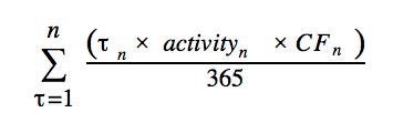
To apply this formula:

1. We first divide the period of interest into n sub-periods. Sub-period n spans Τ days and represents the maximum number of days over which the average activity remains constant and any conversion factors remain constant. 
2. For each sub-period, we multiply the number of days in the sub-period by the average activity for the sub-period and then by the product of the conversion factors for the sub-period. 
3. Next, we divide the sub-period by the period assumed by the benchmarking library (in this case - one year or 365 days).
4. Finally, we sum the prorated results across all sub-periods to yield the total consumption over the period of interest. 

An Example

In this section we’ll apply the formula to actual data to see how it is used in practice. In this example, conversion factors estimate the amount of emissions that would be emitted over a period of one year in units of pounds (lbs.) per square foot (ft²). Refer to the following table:

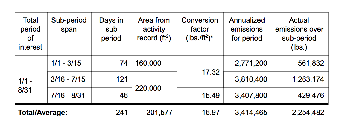
*conversion factors are for 365 days of operation

Looking at this table, we see that the period of interest consists of three sub periods:

1. The first period spans 74 days. During this period, the area is 160,000 ft² and the conversion factor is 17.32 lbs./ft². So, for 74 days, the average annual emissions are 17.32 x 160,000 = 2,771,200 lbs. Since this period lasts only 74 days, the actual emissions for the period are 74/365 x 2,771,200 = 561,832 lbs.
2. The second period spans 121 days. During this period, the area increased to 220,000 ft² but the conversion factor remains 17.32 lbs./ft². So, for 121 days, the average annual emissions are 17.32 x 220,000 = 3,810,400 lbs. Since this period lasts 121 days, the actual emissions for the period are 121/365 x 3,810,400 = 1,263,174 lbs.
3. The last period spans 46 days. During this period, the area is still 220,000 ft² but the conversion factor decreases to 15.49 lbs./ft². So, for 46 days, the average annual emissions are 15.49 x 220,000 = 3,407,800 lbs. Since this period lasts only 46 days, the actual emissions for the period are 46/365 x 3,407,800 = 429,476 lbs.